Many people firmly believe in the prevalence of symmetry in the Universe, leading them to consider the normal distribution as the most suitable, practically default way to approximate the world. Such viewpoint is called ‘Quetilismus’ (named so after Adolphe Quetelet). It is often argued that this belief is merely a matter of having sufficiently large data sizes.
When the distribution of observed data deviates from the normality (or from at least a unimodal symmetry) by exhibiting skewness, it is so often deemed unnatural and difficult to accept by the researchers and some data scientists. In response, many of them strive to ‘manually fix’ the data by ‘symmetrizing’ it, typically by eliminating observations they perceive as outliers or desperately chase for more data (“it must start getting normal, eventually!”). A commonly seen approach is also to transform the data to make it at least ‘appear normal’ eventually, especially during parametric hypothesis testing and regression modeling. These actions stem partially from the misconception that every parametric analysis requires normality (stay tuned for a post debunking this common misconception!) and the false notion that ’non-normal data cannot be reliable or valid’.
The Central Limit Theorem (CLT) is typically invoked to support this claim, by emphasizing the observation of summed or averaged responses from multiple processes. While this is true in many cases, some writers fail to acknowledge the essential assumptions underlying the validity of the CLT. Disregarding these assumptions can lead to slow or failed convergence-in-distribution towards normality. ‘Problematic’ distributions like Cauchy, Levy, power law (Pareto), etc. with heavy tails and/or ’exploding’ moments, which are the no-go-area for the various CLTs are often silently ‘omitted’. One must recognize, however, that these “problematic” distributions play significant roles in various scientific disciplines. For example, the Cauchy (aka Lorentzian) distribution finds application in optics, nuclear physics (spectroscopy), quantum physics (to model the energy of an unstable states), modeling observation of spinning objects (e.g. Gull’s lighthouse 1), modeling the contact resistivity in electronics and even the hypocenters on focal spheres of earthquakes. It is also the solution to the differential equation describing forced resonance in physics. And even though there exists the Generalized Gnedenko-Kolmogorov CLT, helpful with many problematic distributions, but still for certain parametrizations best it can do is the convergence to stable, but not necessarily normal ones.
Another unrealistic assumption when assigning the CLT the dominating role is that it indirectly implies that various factors can act solely in an additive manner (sums), which is not always true. For example, in biology, the skewness naturally arises through the ‘cascades of reactions’, where metabolism and elimination processes can be described in multiplicative manner because of combined activity of enzymes and hormones. Here the product of one reaction serves as the substrate for another, or one hormone activates or inhibits the production/release of another hormone(s). This is why skewed distributions are frequently observed in pharmacokinetics, influenced by various physiological processes this way. Levels of various biochemical markers, even if distributed approximately normally in the population of healthy people, may exhibit extreme skewness in the population of ill patients. The concentration of low-density lipoprotein cholesterol (LDL-C) in patients under severe hypercholesterolemia or the levels of the PSA hormone in oncological patients, (easily spanning 7 orders of magnitude in one direction) serve as excellent examples out of many. Abundance of species, growth of populations or the process of decay make another multiplicative examples of typically skewed distributions. And then we have the product-based Multiplicative CLT (related to the Gibrat’s law) alongside the “classic” additive CLT, leading directly to skewness via log-normality.
There exists a stronger support for the claim that skewness is indispensable part of reality and cannot be disregarded in the scientific description of numerous phenomena. We will mention the multi-agent systems and the first-order kinetics in the context of the Fokker-Planck equation allowing us to derive log-normality from fundamental grounds. Another fundamental source of log-normality is increasing entropy in physical processes. There are scientists, who find the log-normal distributions a “natural distribution” 2. Skewness -not only the log-normal- comes also from the Benford’s law, the time-to-event analysis (nicely picturing the Fisher–Tippett–Gnedenko Extreme Value Theorem), analyzing variables that are naturally bounded near their boundaries (such as age of terminally ill newborns suffering from congenital conditions, complications during birth, or early-life diseases), mixtures of distributions, and the presence of valid extreme observations (outliers).
Now, if we observe and use skewed distributions to describe so many real-world phenomena, it obviously challenges the perception of normality (or even unimodal symmetry) irrespective of sample size or repetition. And the list of areas of science where ’normality is paranormal’ is really long! In light of these considerations, the assignment of normality as the dominant role in science becomes questionable. In other words, the emphasis on normality appears to deny reality or manifests as wishful thinking.`
While delving into resources such as books, papers, tutorials, and courses that describe natural phenomena and statistical analysis methods, one may develop the impression that the Gaussian distribution is abundantly prevalent in nature. It seemingly manifests itself in almost every domain of scientific research, giving the perception that its famous bell-shaped curve is a constant presence in our surroundings.
Or perhaps it is a case of an ‘information bubble,’ where many authors reiterate the same claims, employing identical arguments and presenting the same examples repeatedly? This is not a novel observation and was made about a hundred years ago! It’s remarkable how history repeats itself😊

OK, normality is indeed quite common, and it can be explained, to some extent, on mathematical grounds. We will explore this further in the text. On the other hand, as humans, we are inherently biased in how we perceive patterns and tend to overestimate their frequency subconsciously.
Some people, myself included, have a tendency to believe that red lights are always waiting for them on the road. If we were to objectively count the number of times we actually pass through intersections on a green light, we might be surprised by the results. However, we tend to remember more vividly the instances where we had to wait at red lights. Perhaps a similar bias is at play here as well.
In certain situations normality is very intuitive. Let’s have a look at the weights below. The scratched area reflects the frequency of being chosen by the exercisers. It is evident that most people cannot lift the heaviest weights, and it is also impractical for them to select the lightest weights. Instead, the majority of individuals opt for weights in the middle range, which is easy to imagine without any mathematical analysis—it simply makes intuitive sense. This is one of the reasons why the normal distribution can be so enticing and appealing. 😜

Normal distribution is everywhere, isn’t it?
Maybe that’s why doing workouts releases endorphins and serotonin 😜
Source: Google - Images
The perception of normality is reinforced by our everyday observations of the world around us. We intuitively recognize that certain options or values are more commonly encountered, while others are rarer or exceptionally uncommon.
Take a moment to look at the touchpad on your laptop if you are using one. If your laptop has been in use for several months or longer, you will likely notice a distinct area near the center where it shows signs of frequent touch (possibly slightly shifted to the right if you are right-handed). This region tends to exhibit a rounded shape, reminiscent of an approximate bivariate normal distribution (as you move the cursor both vertically and horizontally).

It turned out that I use my touchpad quite… normally
But there were people in history who extended it to every aspect of humans’ life.
The belief that “normality is everywhere” has a long history that traces back to the 19th century and the work of Adolphe Quetelet. Quetelet, a polymath who excelled in various fields such as mathematics, astronomy, poetry, drama, and sociology, is renowned as the inventor of the Body Mass Index (BMI). He was a staunch advocate for moral and reliable statistical practices and played a crucial role in popularizing the use of the normal distribution to describe human populations3. Quetelet went much beyond the Gaussian Theory of Errors and claimed that normality is the default way of describing the real world.
There have been many opponents of Quetelet’s assumption that humanity can be described by ’normal’ distributions. Francis Edgeworth (1845–1926) said:
The (Gaussian) theory of errors is to be distinguished from the doctrine, the false doctrine, that generally, wherever there is a curve with a single apex representing a group of statistics, that the curve must be of the ’normal’ species". The doctrine has been nicknamed ‘Quetilismus’, on the grounds that Quetelet exaggerated the prevalence of the Normal law.4
Unfortunately, by the time objections were raised, the belief in normality had already gained significant traction and has persisted to this day. In the realm of statistical data analysis, numerous articles, tutorials, and even simplified textbooks either assume normality implicitly or provide seemingly flawless justifications by invoking the Central Limit Theorem (which is justified for additive processes). The prevailing notion suggests that by aggregating cases or treating phenomena as the sum of interventions, normality can be achieved. More sophisticated studies explore deviations from normality to a certain extent and discuss the robustness of various statistical methods (F test in ANOVA, t-test, etc.), ultimately concluding that reliance on normality is generally safe. This fallacious thinking has been embraced by many individuals, including specialists in data analysis. It has become particularly prevalent in the field of data science. Whenever numerical variables are encountered, some individuals thoughtlessly apply the assumption of normality. While this approach may yield satisfactory results in many cases, there inevitably comes a point where it fails to hold true…

The true danger in data analysis
Regrettably, skewness in data is frequently misconstrued as a significant issue, treated as a “challenge to overcome,” something requiring “normalization” and a strenuous struggle. However, it is crucial to acknowledge that skewness is a natural outcome of specific circumstances and underlying mechanisms, which we will delve into in greater depth.
Moreover, the presence of multi-modality and “fat tails” in data further contradicts the notion of “normality reigns”. Unfortunately, this aspect is often disregarded and overlooked. When combined with the aforementioned asymmetry, these factors sufficiently undermine the concept of “omnipotent normality.”
However, until these realities are acknowledged and embraced, Quetilismus will be alive and well.
Ultimately, we can come across countless examples of normality in nature, accompanied by an abundance of amusing (and funny) pictures on the Internet. We even encounter it within the realm of quantum mechanics, which effectively ‘governs’ our lives on the macro-scale. All of this leads us (or at least tempts us) to believe that normality dominates in the Universe. But is this belief grounded in reality?

However, if the dominance of the Central Limit Theorem (CLT) and the exclusive reliance on “sums over thousands of sub-processes” were the sole driving force, then the occurrence of observed skewness would indeed be rare, wouldn’t it? We wouldn’t need to concern ourselves with skewed distributions as we currently… DO.
Yet, the reality is that we observe skewness in numerous contexts. Isn’t the “Box-Cox” transformation, including the logarithmic transformation, a frequently discussed including the logarithmic transformation, a frequently discussed (and deservedly criticized!) topic on statistical forums? 😜
So, what is happening? Does the CLT fail? But remember, it is a theorem that always “works” as long as certain assumptions hold! Is there something more to the universe beyond symmetry alone? Well, it is a clear indication of processes and laws that disrupt the dominance of symmetry and normality. In the following sections, we will explore some of these processes and laws, and we will discover the widespread presence of skewness in nature.
Oh, and let us not forget that quantum physics benefits from power-law distributions too. They are used to describe phenomena such as the distribution of energy levels in complex systems, the behavior of quantum field fluctuations, and the statistics of entanglement in many-body systems. Power-law distributions inherently exhibit skewness and deviate significantly from the bell-shaped Gaussian distribution. So - the ’normality solely controls the world at the quantum level’ argument fails.
Before we dive into the details, it’s important to clarify the terms “additive” and “multiplicative.” Additivity is associated with symmetry, while multiplication is associated with asymmetry. Let’s explore this concept with some examples.
When we add or subtract a number from a fixed value x, both sides of x are affected equally, distanced from x by the same number of units. The added or subtracted value is not “weighted” in any particular way, and the results can be either positive or negative, depending on the operation and the magnitude of the added value.
In contrast, when we multiply or divide a fixed value x by a number, the effect on both sides of x is not equal. For example, dividing x by 2 results in a value that is half of x, while multiplying x by 2 results in a value that is double x. The effect of the multiplication or division operation is not symmetric, and the results can only be of the same sign as the input value regardless of the magnitude of the multiplier (provided the multiplier is positive!).
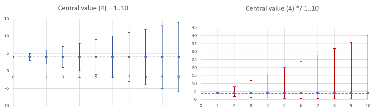
Adding / subtracting values result in symmetry. Multiplication / division - in asymmetry
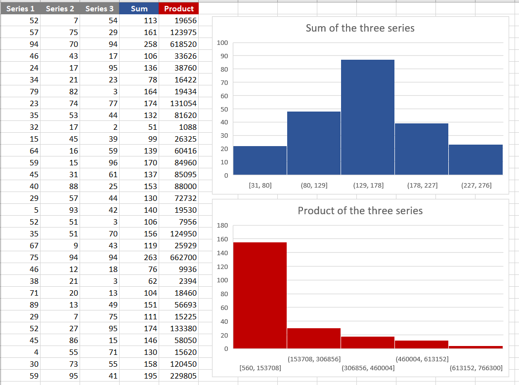
Summing series produces a new series in which the resulting values are symmetrically scattered around a central value (mean or median). The occurrence of extreme values on both sides of the distribution is approximately equal. When the series are independent, the frequency of extreme values is expected to be smaller than the frequency of more “typical” values. As the number of series increases, this distribution takes the familiar shape we recognize as a “pyramid”, approaching the “bell”. This example demonstrates the basic workings of the Central Limit Theorem. We will delve into this topic further in the following sections.
Remark: This also explains why the arithmetic mean, being an additive measure, is a useful summary of central tendency for symmetrically distributed data. However, in the case of highly skewed data, although the arithmetic mean can still be calculated, it may not provide a meaningful measure.
Multiplication of such series results in a new series where the resulting values exhibit strong asymmetry around a ‘central’ value. Here, you might recognize the simplistic concept of the Multiplicative Central Limit Theorem. (OK, far from ideal, but gives some clues).
Adding/subtracting values result in symmetry. Multiplication / division - in asymmetry
Before we go deeper into the concept of skewness, let’s take a moment to reconsider the claim regarding the prevalence of the normal distribution in nature. In numerous sources, one can find a justification along the lines of: ’the observed data (a random variable) generated by the phenomenon under investigation is often an outcome of many components that interact additively (sums of components). As per the Central Limit Theorem, this leads to the emergence of the widely observed approximate normal distribution.’
We will not repeat statistical textbooks regarding the different formulations of the Central Limit Theorem, only recall:
Now, if the relevant conditions are satisfied, then for a set of independent random variables, the sum of standardized variables converges in distribution to the standard normal distribution as the number of input variables approaches infinity.
To illustrate this, let’s conduct some simulations and discuss the results. We will start with a simple yet remarkable example. By applying the classic CLT to a set of IID random variables, we can observe the transformation of noticeably skewed “components” into a nicely shaped bell curve of their sum. We will deliberately choose asymmetric distributions to make things more difficult.
Here we will make a remark, that the process of summation of the independent random variables is just a convolution of their probability density functions. We know the results of convolutions of many several distributions. For example, utilizing the gamma distribution:
$$ \sum_{i=1}^n \Gamma(\alpha_i, \theta) ~\text{\textasciitilde}~\Gamma(\sum_{i=1}^n\alpha_i,\beta) ~~~ \alpha_i>0, \beta>0 $$
Note: Do not get confused! There are two equivalent ways of parameterizing the gamma distribution:
- shape: α or k and rate: β=1/θ ; then mean=α/β and variance=α/β^2
- shape: α or k and scale: θ=1/β) ; then mean=αβ and variance = αθ^2
In R, the default parametrization is shape (α) and rate (β). Pay attention to the parametrization or the calculations will not agree. Sometimes also the main parameters are swapped, like here: http://www.math.wm.edu/~leemis/chart/UDR/PDFs/GammaNormal1.pdf
Why did we select the gamma distribution for this demonstration? Firstly, because the gamma distribution is closed under convolution, meaning that the sum of gamma-distributed variables follows the gamma distribution. Secondly, by appropriately parameterizing the ‘component’ variables, we can introduce visible skewness to the resulting components. We will see that the resulting distribution will be almost indistinguishable from the normal one, because the limiting distribution for Γ(shape [α], rate [β]) for large value of the shape parameter (α) is the normal distribution parametrized as: N(α/β, √(α/β^2)) 67 .
Regardless of different supports, the beta, (generalized) gamma, and log-normal distributions are mathematically related and may resemble each other by shape under specific parametrizations. For this reason, some phenomena are sometimes analysed using either the log-normal or the gamma or beta distributions (except specific scenarios where the three differ). It is worth remembering, that the log-normal is a limiting distribution for the generalized gamma.
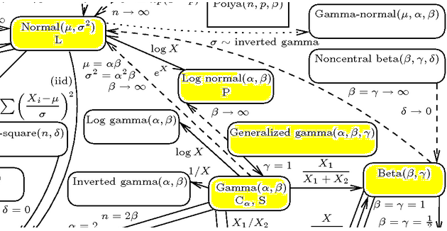
Part of the interactive diagram: http://www.math.wm.edu/~leemis/chart/UDR/about.html
For 15 samples (the initial seed was recorded; N=100) from the Γ(1, 15) distribution:
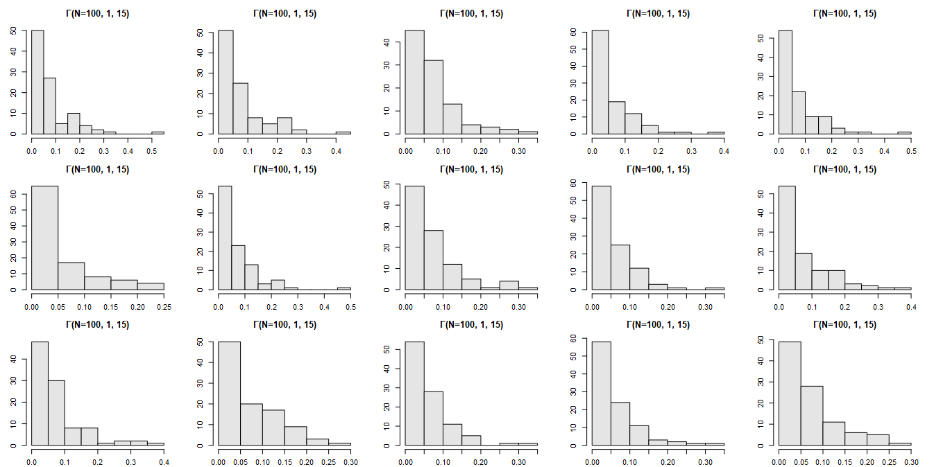
We will sum these highly skewed components and observe the result…
As expected, after summation (no need to scale - just convolve) we obtain Γ(15, 15) ≈ N(15/15=1, √(15/15^2)≈0.26):
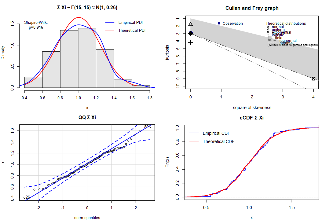
The Central Limit Theorem at its best!
OK, the CLT manifested itself resulting in almost perfect normal distribution, even if many component factors were visibly skewed.
Now let us see what will happen if we sum up 15 various normalized distributions of different shapes:
The set of distributions will be sampled with replacement. We will deliberately skip the normal distribution to make it more difficult for the CLT. We will count on the Lyapunov CLT without checking the relevant condition.
The distributions of the ‘components’:
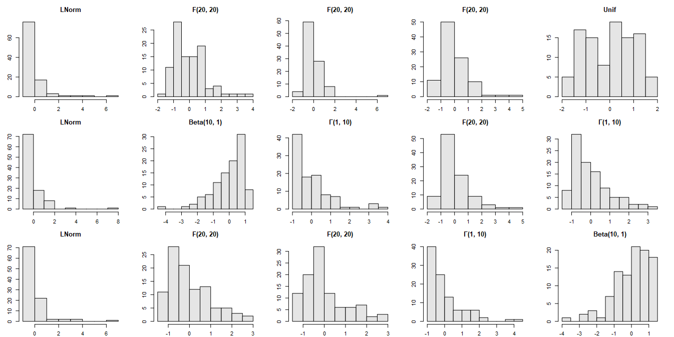
Let’s complicate the task with different shapes of the input distributions
And the result:
Again - quite a nice convergence towards normality!
The results confirmed the expectations. The convergence of the sum of the components in distribution to the normal one is well visible.
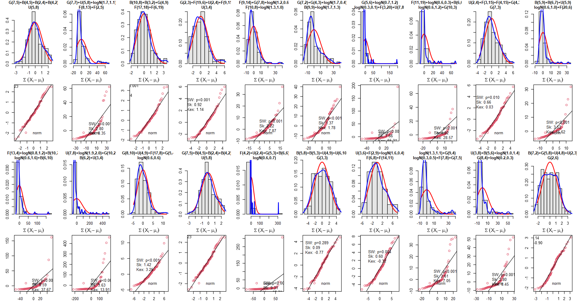
In the last simulation we will observe a completely free-ride, still employing the Lyapunov CLT. We will define 5 types of distributions with randomly selected parameters:
Then 5 distributions will be sampled with replacement, scaled, and summed up. Parameters of these distributions will be sampled as well from the listed ranges. The sampling will be repeated 20 times using different seeds. The results will contain both the histogram with kernel estimator of the empirical density, theoretical density of the normal distribution (with parameters estimated from the sample), Quantile-Quantile plot (for the normal distribution), estimators of skewness (should be 0 for ideal normality) and Excess-Kurtosis (should be 0 for ideal normality) followed by the Shapiro-Wilk test of non-normality.
The specification of the sampled distributions is placed in the titles of histograms.
The results: Now that’s totally a ‘free ride’!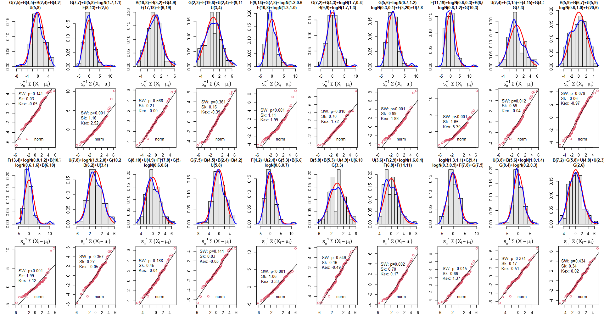
Conclusions:
Despite the challenging conditions employed, the distribution of the sum demonstrated convergence towards normality, rendering it indistinguishable from the normal distribution in 50% (10) of cases according to the Shapiro-Wilk test.
Although the Shapiro-Wilk test rejected normality in some cases, the resulting distribution exhibited notable symmetry and closely resembled normality in the majority of instances. The points in the QQ plot aligned closely with the straight line, with only a few outliers or deviations observed. However, it is important to note that non-normality tests tend to be idealistic and gain power with larger sample sizes, often rejecting the null hypothesis even for minor deviations from their theoretical assumptions. One notable challenge was observed with kurtosis. It is reasonable to anticipate improved results by including more than just 5 distributions in the analysis.
Remarkably, these results were achieved without explicitly checking the Lyapunov condition. The utilization of “good distributions” sufficed for the analysis, as there is no “virtual checker” in reality to verify these conditions on our behalf.
So far, we have demonstrated that the Central Limit Theorem can indeed account for the pervasive presence of normality in nature, particularly when the observed phenomena are the mean (sum) of underlying sub-processes. But what about the situations when it does not?
First and foremost, it is important to acknowledge that in the idealized simulations we conducted, we assumed that all the necessary conditions were satisfied:
We made the assumption that the required moments of the distributions were finite. However, in reality, the finiteness of these moments is an inherent property of a process and cannot be verified or checked by anyone. Furthermore, it is possible that one or more ‘components’ exhibit properties similar to the Cauchy, Levy, or similarly ‘difficult’ distributions, as discussed in the introduction chapter. As mentioned earlier, for certain parametrizations the Generalized Gnedenko-Kolmogorov CLT, while helpful with many problematic distributions, may offer convergence only to stable, but not necessarily normal distributions.
We did not explicitly verify the Lyapunov condition on higher moments, but instead chose distributions that were considered “nice” and likely to satisfy those conditions. In reality such rigorous selection of distributions is of course unrealistic.
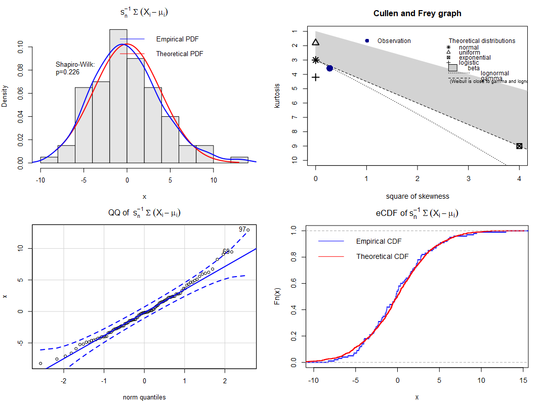
We standardized the random variables. Without that there is no guarantee of convergence to normality, except for trivial cases like the gamma distribution example. To illustrate this, we reran the simulation without standardization, using the same seeds. As a result, the QQ-plots did not exhibit the same favorable outcomes as before. While some symmetric distributions were still present, they were noticeably less frequent.
We focused on scenarios where the component processes acted additively, resulting in the observed mean responses as sums of standardized variables. However, it is essential to recognize that this assumption is not universally applicable to all natural phenomena. In reality, there are processes that act multiplicatively, and their effects may manifest differently. The consideration of multiplicative processes and their mixtures introduces a different perspective and may lead to alternative distributions and behaviors that deviate from the conventional expectations of the Central Limit Theorem.
We made so many assumptions, while neither can be guaranteed by the real phenomena! In reality everything ‘just happens’, without ‘considerations’.
Without scaling it does not look that good!
These observations emphasize the importance of considering the specific conditions and assumptions when applying the Central Limit Theorem in real-world scenarios. This works in simulations, because we are the ones who choose the distributions. And we did not even consider dependency in variables - something that cannot be ruled out in reality.
As we mentioned earlier, it is not universally assumed that all factors affecting an observed process must act additively. In certain domains such as pharmacokinetics, random influences like cascade enzyme activity, diffusion, permeation, and flow rates have a multiplicative effect on the clearance of substances. This results in complex drug concentration-time profiles that are predominantly characterized by skewness, with log-normality and mixtures being prevalent.
Now, let us explore what happens when we replace summation with product. We have already observed this phenomenon earlier in this article. Multiplication tends to introduce skewness. We will now examine the Multiplicative Central Limit Theorem (sometimes related to the Gibrat’s law). In this case, we will utilize the Lyapunov CLT, which allows for different distributions. However, we still require the random variables to be independent, positive-valued, and have finite variance of the squared variable (i.e., square-integrable density function), which holds for the distributions employed in our simulations. Under these conditions, the product of random variables converges in distribution to the log-normal distribution.
To assess the normality of the results, we will repeat the previous simulations by replacing summation with the product and then take the logarithm of the result (i.e., shapiro.wilk(log(X))). We will not center the variables after scaling to avoid negative values. If the data can be closely approximated by a log-normal distribution, then assessing the normality of log-transformed values (log(N)) will serve as a confirmation.
For the same set of input distributions as previously:

We got the following results:
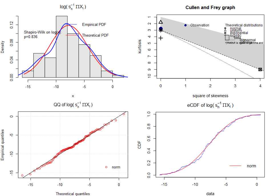
The log-normality is confirmed very well!
The approximate log-normality was confirmed satisfyingly on the log-scale. Of course, deviations from the theoretical pattern exist for exactly the same reasons as before. On the original scale, the deviations from the patterns are more visible (larger values), but still looking good.
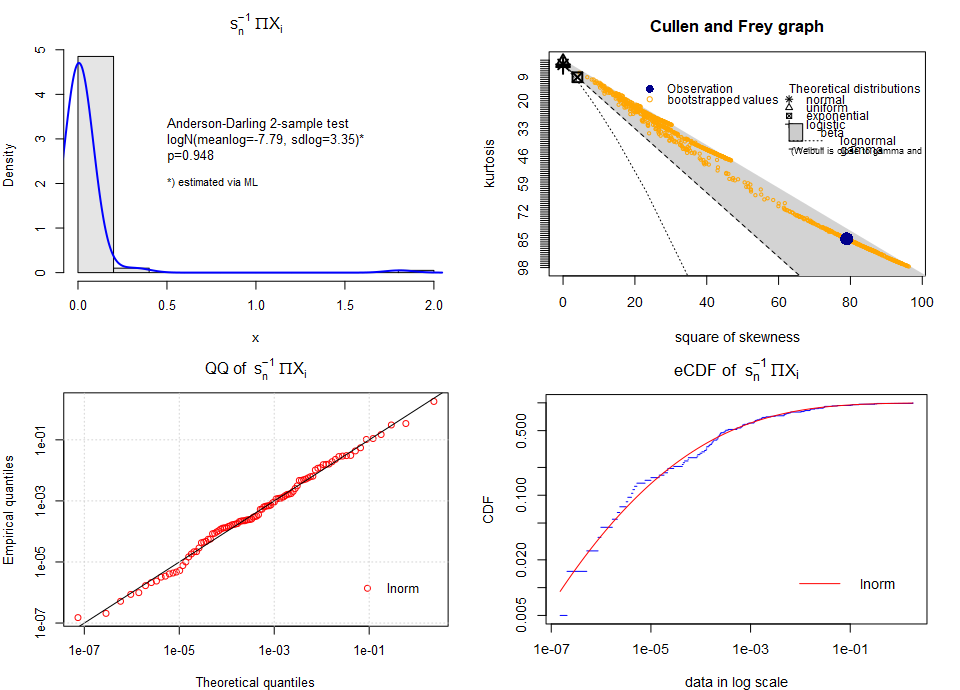
Achieved log-normality on the original scale
Here the Cullen-Frey placed the distribution in the zone representing the beta distribution rather than on the line representing the log-normality, but this a common issue when differentiating skewed distributions only in the [kurtosis – skewness squared] space. Actually, it is difficult for the plot to locate the empirical distribution even if the data were sampled from the log-normal distribution itself. At least it places the distribution in the “zone of skewness”, as expected. Majority of the bootstrapped points representing the distribution are located much closer to log-normality3.
Let us conduct another round of simulations using the previously sampled distributions with sampled parameters, but this time utilizing multiplication instead of summation (without centering). As we can see, the approximate log-normality was demonstrated very well.
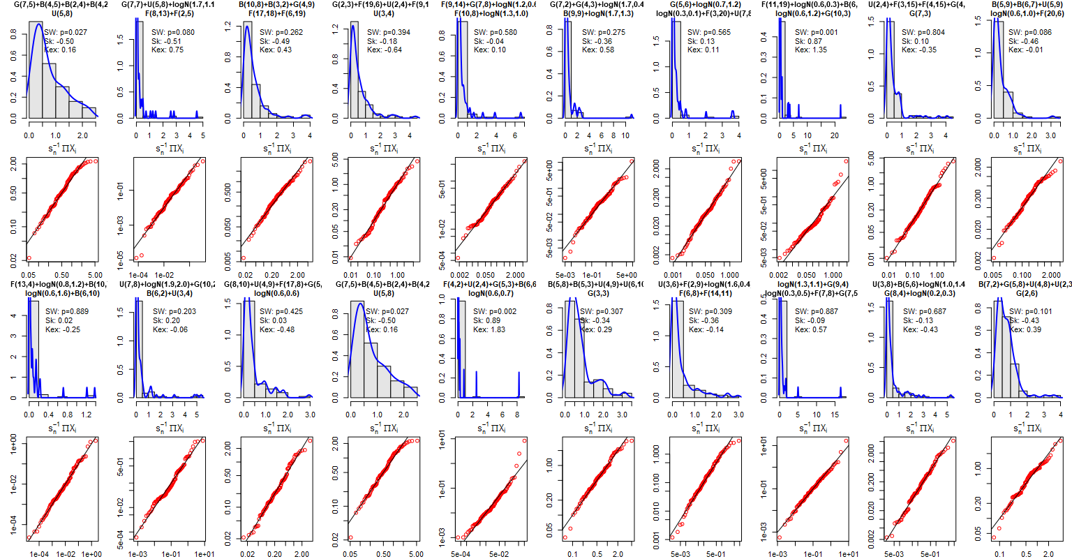
Looks good!
So far, we have discussed and partially demonstrated that skewness can arise from various factors, including:
Our simulations were idealized, combining the random variables either in additive or multiplicative way. In reality, a process may be affected by multiple factors in both manners, resulting in asymmetric distributions not adequately described by the log-normal or normal distributions.
The above points are not the only source of skewness in nature.
Skewness can arise from a multitude of factors, often working together in mysterious ways. While we have explored some mathematical explanations for the presence of both symmetry and skewness in nature, it is important to consider the deeper sources that underlie these phenomena. In the following sections, we will examine and discuss selected factors that can serve as the fundamental sources of skewness. By delving into these underlying mechanisms, we can gain a deeper understanding of the complex nature of skewness and its manifestations in various domains.
It is commonly taught that skewness is likely to occur, if mean values are low, variances are large, and values cannot be negative. This constrains us only to positive skewness, so let us replace the last observation instantly with “values are bounded at one side”*.
* Actually, this is a simplification, as values of numerous real variables are typically bounded at both sides. In the analysis, however, we typically care of only one side, “closer” to the analyzed phenomenon. For example, age cannot be negative, but – for humans – it is definitely smaller than, say, 260 years (if we assume that the oldest man in history, Li Qingyun, really died at 256). This does not invalidate our considerations, though. If we speak about mortality (due to some terrible disease) in newborns, we typically deal with right (positive) skewness with data truncated at 0 days (ignoring the upper bound). Conversely, when we analyze data of mortality in elderly, the skewness will be typically negative (left), with truncation point at, say, 100 years (ignoring the lower bound).
A few examples:
Counts. Counts are positive, integer values truncated at zero. Two corresponding topics are: Poisson and negative binomial distribution and the Benford’s law of prevalence of small numbers under certain conditions.
Age of newborns suffering from a terminal age-specific disease. The older the baby the lower probability of getting ill. This results in right-skewed distribution, sharply truncated at 0.


Naturally bounded variables can be intriguing…
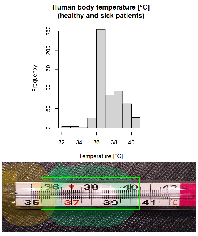
Mixtures of distributions can naturally form skewness. A typical example is a mixture of (approximate) normal distributions with some mean-variance relationship, typically – the larger the mean the larger the variance. Below we can observe such case – three normal distributions of different location and spread form a skewed one on the right.
Note, that the from the three distributions were concatenated, not summed. Looking only at the right one (this is what we will see in nature) we have no prior knowledge of the actual number of elements in each group unless we have generated them.
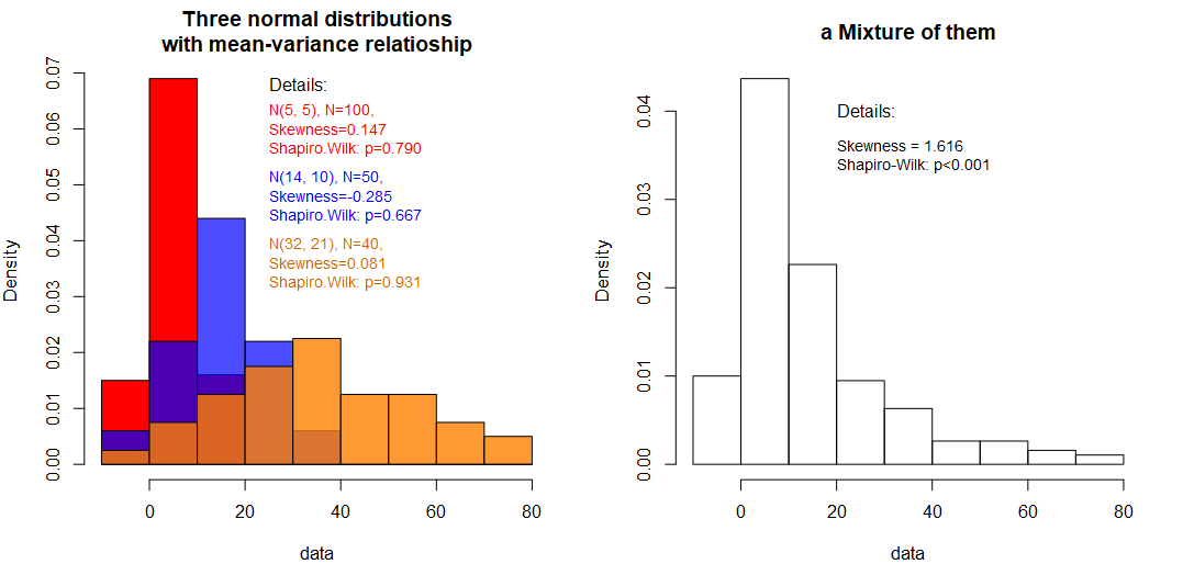
Interacting processes can create mixtures of distributions
In some cases, mixtures can be effectively separated during the analysis. If analysts have prior domain knowledge suggesting the presence of a discriminatory categorical factor, they can include this factor as a covariate in their model. By doing so, the mixture can be divided into approximately symmetric and homogeneous groups.
This provides an explanation for the emergence of a virtual skewness in the data, which can occur when certain factors that could potentially differentiate groups are overlooked. Frequently, we may not even be aware that such factors exist, leading to the treatment of inseparable mixtures as a single entity.
Automated methods for separation also exist, but they tend to be purely mechanistic and may create divisions that lack meaningful interpretation, solely based on statistical properties. An example of such naïve separation can be seen below, where the left part is separated based on its symmetry. However, it is important to note that this separation still represents a mixture.
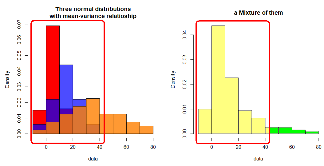
Attempts to separate them naively can be misleading
Skewness can also arise due to valid observations that are located far from the central tendency, commonly referred to as outliers. These outliers have a significant influence on the distribution, pulling it towards the direction of their extreme values and contributing to its skewness.
Many tutorials often refer to the “3 sigma” rule, which states that any observation located farther than 3 times the standard deviation (σ) from the mean is considered an outlier. This rule is derived from the properties of the Normal distribution, where the interval of mean ± 3xSD encompasses approximately 99.7% of all observations. However, this rule is specific to the Normal distribution and may not be appropriate for non-normal ones. Alternatively, the Chebyshev inequality can be used as it is more general and applicable to any distribution. It provides a more “liberal” criterion for identifying outliers. For example, it states that within any distribution, at least 88.9% of the data will fall within 3 standard deviations from the mean, 96% within 5 standard deviations, and 99% within 10 standard deviations.
Outliers can be classified into two categories: errors and valid observations. In the case of valid observations, outliers can be either single data points that are not representative of the majority or a group of observations that exhibit a unique property inherent to the phenomenon being investigated. Excluding valid outliers from the analysis can lead to false conclusions and incorrect decisions.
In certain contexts, such as fraud detection, outliers play a crucial role in analyzing and understanding the data. They can serve as indicators of new discoveries, warnings before disasters (as seen in the tragic “Flint Water Crisis” where high concentrations of lead were ignored and resulted in loss of lives), announcements (e.g., malfunctioning sensors), violations of procedures, omitted categorical covariates in a model, or simply reflect the natural and inherent properties of the investigated process, influenced by human factors.
Recognizing the significance of outliers and their potential implications is essential for conducting thorough analyses and drawing accurate conclusions in various domains.
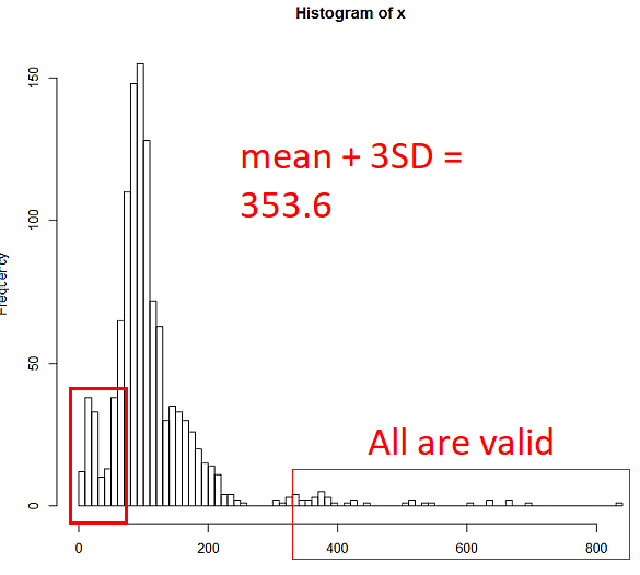
In the field of clinical biochemistry, it is not uncommon to encounter valid outliers that deviate significantly from the mean, sometimes even by several orders of magnitude. This is particularly observed in datasets that involve measurements of biomarkers or substances with wide concentration ranges. An example of such a dataset is the concentration of prostate-specific antigen (PSA) in oncological patients.
In the given dataset, the largest valid value of PSA (1500) is approximately 7 orders of magnitude larger than the smallest value (0.001). This wide range of values reflects the inherent variability in the clinical state within the patients population.
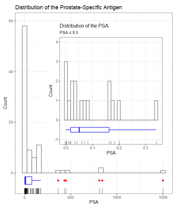
Some clinical markers can span several orders of magnitude!
The individual “human factor” plays a crucial role in healthcare outcomes, as it introduces a significant level of unpredictability and leads to diverse responses to treatment among patients. When analyzing data from patients collectively, we often observe a wide range of patterns, including multiple modes, strong skewness, and extreme outliers.
The complexity of the “human factor” arises from a multitude of interconnected sub-factors. Thousands of chemical reactions occur within our bodies every second, and any disruptions or failures in these reactions can have an impact. Furthermore, numerous environmental conditions such as temperature, humidity, air pressure, and pollution can influence our physiological responses. Personal habits, including smoking and drinking, dietary choices, hydration status, medications and their interactions, surgical procedures, illnesses, infections, allergies, deficiencies, and overdosing of drugs all contribute to the intricate web of factors affecting our health. Additionally, our DNA and its mutations, which can be caused by factors like radiation and mutagens present in our environment (such as carcinogenic substances in food and water), have a significant influence. Hormonal and enzymatic activity, stress levels, lifestyle (ranging from sedentary to highly active or extreme), familial burdens, and even the placebo and nocebo effects all add further complexity.
Processes within the human body, such as the pharmacodynamics of a drug can be sensitive to the initial and boundary conditions, which is reflected by the differential equations used to describe them. These equations can exhibit instability under specific conditions, further adding to the variability of individual responses to therapies.
Considering the multitude of biological and physical factors at play, it becomes evident that different patients may exhibit entirely distinct reactions to the same therapy. This complexity is not limited to healthcare but can also be observed in other fields such as sociology and economics, where the interactions of various factors give rise to diverse outcomes and behaviors. This reflects the mixed responses observed among individuals due to the diverse interactions and influences of the various sub-factors. In such cases, the data may exhibit distinct clusters or subgroups with different characteristics and patterns, reflecting the heterogeneity of the underlying processes.
The complexity of the reactions in living organisms can create complex mixtures!
The survival time, or the time to a specific event, often exhibits skewed data patterns, and this can be shown in a beautiful manner!
Let us focus on the “time to the first event”. We record the time for each subject until the event of interest occurs, at which point we stop counting. This represents the maximum time without experiencing the event for each subject.
Interestingly, there exists a theorem known as the Fisher-Tippett-Gnedenko Extreme Value Theorem, which provides a mathematical framework for understanding the behavior of extreme values. This theorem has several applications in fields such as finance, environmental science, engineering, and reliability analysis. It establishes certain conditions under which the maximum value in a sequence of independent and identically distributed random variables, after appropriate normalization, converges in distribution to one of three limiting distributions: the Gumbel distribution, the Fréchet distribution, or the Weibull distribution. All the three can exhibit a noticeable skewness (for Weibull - both left and right).
It does not claim that the normalized maximum values eventually converge in distribution, BUT if they do, the limiting distribution is either of the three mentioned above. By the way, when the shape parameter of the Weibull distribution is set to 3, it closely resembles the normal distribution.
This does not end the list! Exponential, gamma, log-normal, and log-logistic distributions are also commonly used in the time-to-event analysis.
There is another, less mathematical explanation of how the skewness may emerge in the survival analysis. Let’s consider the nature of the event of interest, ignoring loss to follow-up, and identify three scenarios:
Early effect: In this scenario, the event of interest occurs predominantly soon after recruiting patients, and its frequency decreases noticeably over time, resulting in sporadic occurrences. This creates a right-skewed asymmetry in the data. An example of this could be death following a transplantation, where patients who survive the first few days have higher chances of long-term survival. In other words, their condition stabilizes after an initial critical period.
Delayed effect: In contrast to the early effect, the frequency of the event of interest increases later in time. This typically occurs when patients experience the event due to a progressing illness that is resistant to treatment or a breakout phenomenon that is more likely to happen after a certain number of days. This leads to left-skewed asymmetry in the data, as the event becomes more frequent as time progresses.
We can also mention the third simple case: the uniformly distributed effect, where the event of interest occurs uniformly over time, with no clear preference for a specific period. This may result in a symmetric distribution, but not necessarily the normal one. /
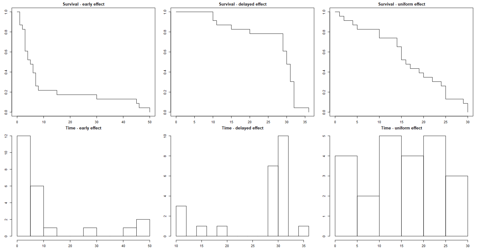
Survival time a classical example of (usually) skewed distribution
Benford’s Law is a fascinating phenomenon that exemplifies the presence of skewness in real-world datasets. It observes that in various collections of numbers, such as mathematical tables, real-life data, or their combinations, the leading significant digits do not exhibit a uniform distribution as expected, but instead display a strong skewness towards the smaller digits. Benford’s Law states that the significant digits in many datasets follow a log-normal distribution8.
This law has numerous applications, including fraud detection, criminal investigations, social media analysis, genome data analysis, financial investigations, and macroeconomic data analysis, among others. Additional information can be found in 9 and 10. It is important to note that there are also significant counter-applications of Benford’s Law, such as its use in analyzing election data under specific conditions11.
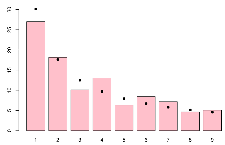
Distribution of first digits (in %, red bars) in the population of the 237 countries of the world as of July 2010. Black dots indicate the distribution predicted by Benford’s law. (source Wikipedia)

Another illustration of the Benford's law (source Wikipedia)
This is another beautiful manifestation of mathematics in our everyday life (including our organisms). While was really tempting to start from this topic and make it the king of this article, I decided to leave the best for last (almost) 😊
Exponential kinetics is a term describing a process, in which the rate of creating (concentrating) or losing some substance or property is proportional to the remaining amount of the substance. A constant proportion (not amount!) of something is processed per unit time. Or differently - the greater the amount of something, the faster the process.
$$ \frac {dC} {dt} = -kC~~~~\tiny(E1) $$
Because of the exponential form of the solution to the above equation:
$$ C = C_0~ e^{-kt}~~~~\tiny(E2) $$
The process is called “mono-exponential rate process” and represents exponential decay or concentration over time.
There is some name confusion surrounding this topic. The kinetics is referred to as both linear (in the context of the differential equation) and exponential (referring to the concentration over time). It’s important to note that both terms actually pertain to first-order kinetics and essentially convey the same meaning, with the specific usage depending on the context.
The zero-order kinetics is about processing the same amount of something regardless of its concentration. The first-order kinetics is about processing the same fraction of something.
One of the common places where it naturally occurs is the process of radioactive decay. Another important application of it is the pharmacokinetics of medicines, namely the elimination of a medicine from organism 12. The elimination here depends on the concentration of the medicine (called reactant) - the rate of elimination is proportional to the amount of drug in the body. The majority of drugs are eliminated in this way, making it an important theoretical model assuming “clear situation”, that is to say – no “modifiers” can affect the process.
The above examples assumed “constant value of the constant k”. While it is reasonable for the radioactive decay (allowing us to calculate the half-life: t½~=0.693/k), the elimination of medicines may strongly depend on many factors: interactions with other drugs and human factor (described earlier sum-product of many factors). In this case, the constant “k” may vary.
The equation (E1) turns into a stochastic differential equation:
$$ d[X]/dt=−(μ_k~+σ_k~η(t))[X] ~~~~\tiny (E3) $$
where μ_k is the mean reaction rate and σ_k is the magnitude of the stochastic fluctuation. The function η(t) describes the time-dependency of the random fluctuations (with amplitude 1), which we here assume to be independent and identically normally distributed. Fluctuations of η(t) will result in fluctuations of the solution for the equation (E3), which creates a random variable. The equation that describes the temporal evolution of the PDF of this variable is the Fokker–Planck equation 13. It turns out, that the solution of the Fokker-Planck equation derived from the equation (E3) is the PDF of the log-normal distribution, with parameters μ and σ. 14
Briefly, the first-order kinetic model with randomly fluctuating sink/concentration rate is a potential source of the log-normality in nature. Isn’t this beautiful? Think how widespread is this mechanism practically everywhere in physics, chemistry, biology!
The best I left for the end In the previous section I mention part of drug pharmacokinetics. What if I told you that similar mechanisms are much more widespread?
The mentioned Fokker-Planck-type equations naturally link with the theory of multi-agent systems, used to describe human activities and economic phenomena.
Let’s consider a certain specific hallmark of the population of agents. The hallmark is measured in terms of some positive value “w”. The agents have the objective to reach a target fixed value of “w” by repeated upgrading. This corresponds to microscopic interactions. The upgrade of the actual value towards the target is different, depending on the actual state of the agents, it’s dynamic. This leads to the same problem and a similar solution described in the previous chapter.
This is truly deep, because there is a well-established connection between kinetic modeling of social and economic phenomena with classical physical kinetic theory of rarefied gases, providing advanced analytical tools for this class of problem. That is to say, the collective behavior of a group of large number of individual agents is described using the laws of statistical mechanics, as if it was a physical system composed of many interacting particles.
Detailed discussion with complex mathematical derivations and rich domain-related literature can be found in 11.
Another way to infer log-normality from fundamental laws is to refer to entropy. Fluctuations in open-system processes (exchanging both energy and matter with its surroundings) in their evolution toward more probable states yield multiplicative variations about the mean. The non-linear dispersion of thermodynamic states, i.e. matter and energy defined by chemical potentials, underlies the skewness.
Details can be found in 2, where the authors call the log-normal distribution the “Natural Distribution”, coming from physical processes with conserved positive quantities.
To appreciate the widespread presence of skewness in nature, let us explore several examples across different domains where skewness, often expressed in terms of the log-normal distribution, plays a significant role. Following that, we will briefly list a selection topics and examples of research papers that describe and analyze skewness within specific scientific fields. The examples do not link entirely to log-normality, but also to gamma, Weibull, and other skewed distributions (e.g. https://en.wikipedia.org/wiki/Weibull_distribution#Applications ).
… and many more!
Let us link to a number of available papers:
Geology and mining
📖 Singer D. A., The lognormal distribution of metal resources in mineral deposits, Ore Geology Reviews, Volume 55, 2013, Pages 80-86, ISSN 0169-1368,
https://doi.org/10.1016/j.oregeorev.2013.04.009 ,
https://www.sciencedirect.com/science/article/pii/S0169136813001133
Biology and biophysics
📖 Furusawa C, Suzuki T, Kashiwagi A, Yomo T, Kaneko K. Ubiquity of log-normal distributions in intra-cellular reaction dynamics. Biophysics (Nagoya-shi). 2005 Apr 21;1:25-31. doi: 10.2142/biophysics.1.25. PMID: 27857550; PMCID: PMC5036630.
https://www.ncbi.nlm.nih.gov/pmc/articles/PMC5036630/
📖 D.Fraga, K.Stock, M.Aryal, et al., Bacterial arginine kinases have a highly skewed distribution within the proteobacteria, Comparative Biochemistry and Physiology, (2019), Part B,
https://doi.org/10.1016/j.cbpb.2019.04.001 ,
https://www.sciencedirect.com/science/article/abs/pii/S1096495919300831?via%3Dihub
Epidemiology
📖 Saltzman BE. Lognormal model for determining dose-response curves from epidemiological data and for health risk assessment [published correction appears in Appl Occup Environ Hyg 2001 Oct;16(10):991]. Appl Occup Environ Hyg. 2001;16(7):745-754. doi:10.1080/10473220121485,
https://pubmed.ncbi.nlm.nih.gov/11458922/
Stock market
📖 I. Antoniou, Vi.V Ivanov, Va.V Ivanov, P.V Zrelov, On the log-normal distribution of stock market data, Physica A: Statistical Mechanics and its Applications, Volume 331, Issues 3–4, 2004,Pages 617-638, ISSN 0378-4371,
https://doi.org/10.1016/j.physa.2003.09.034
Pharmaceutical industry
📖 Meiyu Shen, Estelle Russek-Cohen & Eric V. Slud (2016):Checking distributional assumptions for pharmacokinetic summary statistics based onsimulations with compartmental models, Journal of Biopharmaceutical Statistics, DOI:10.1080/10543406.2016.1222535
📖 Lacey LF, Keene ON, Pritchard JF, Bye A. Common noncompartmental pharmacokinetic variables: are they normally or log-normally distributed?. J Biopharm Stat. 1997;7(1):171-178. doi:10.1080/10543409708835177
Clinical biochemistry and laboratory diagnostics
📖 Feldman M, Dickson B. Plasma Electrolyte Distributions in Humans-Normal or Skewed?. Am J Med Sci. 2017;354(5):453-457. doi:10.1016/j.amjms.2017.07.012,
https://pubmed.ncbi.nlm.nih.gov/29173354/
📖 Campbell D J, Hull E.W., Does serum cholesterol distribution have a log- normal component?
📖 Kletzky OA, Nakamura RM, Thorneycroft IH, Mishell DR Jr. Log normal distribution of gonadotropins and ovarian steroid values in the normal menstrual cycle. Am J Obstet Gynecol. 1975;121(5):688-694. doi:10.1016/0002-9378(75)90474-3
📖 Distler W, Stollenwerk U, Morgenstern J, Albrecht H. Log normal distribution of ovarian and placental steroid values in early human pregnancy. Arch Gynecol. 1978;226(3):217-225. doi:10.1007/BF02108902
Ecology & Environment
📖 Ogana, F. & Danladi W. (2018). Comparison of Gamma, Lognormal and Weibull Functions for Characterising Tree Diameters in Natural Forest.
📖 Cho, H., Bowman, K. P., & North, G. R. (2004). A Comparison of Gamma and Lognormal Distributions for Characterizing Satellite Rain Rates from the Tropical Rainfall Measuring Mission, Journal of Applied Meteorology, 43(11), 1586-1597. Retrieved Jun 29, 2022,
https://journals.ametsoc.org/view/journals/apme/43/11/jam2165.1.xml
📖 Iaci, Ross Joseph, "The gamma distribution as an alternative to the lognormal distribution in environmental applications" (2000). UNLV Retrospective Theses & Dissertations. 1206.
http://dx.doi.org/10.25669/z0ze-k42y ,
https://digitalscholarship.unlv.edu/cgi/viewcontent.cgi?article=2205&context=rtds
Sociology
📖 Yook, S. H., & Kim, Y. (2020). Origin of the log-normal popularity distribution of trending memes in social networks. Physical Review E, 101(1), [012312].
https://doi.org/10.1103/PhysRevE.101.012312
Physics
📖 Grönholm T, Annila A. Natural distribution. Math Biosci. 2007;210(2):659-667. doi:10.1016/j.mbs.2007.07.004,
https://www.mv.helsinki.fi/home/aannila/arto/naturaldistribution.pdf
Interdisciplinary
📖 Andersson, A. Mechanisms for log normal concentration distributions in the environment. Sci Rep 11, 16418 (2021).
https://doi.org/10.1038/s41598-021-96010-6 ,
https://www.nature.com/articles/s41598-021-96010-6
📖 Limpert E., Stahel W. A., Abbt M., Log-normal Distributions across the Sciences: Keys and Clues: On the charms of statistics, and how mechanical models resembling gambling machines offer a link to a handy way to characterize log-normal distributions, which can provide deeper insight into variability and probability—normal or log-normal: That is the question, BioScience, Volume 51, Issue 5, May 2001, Pages 341–352,
https://doi.org/10.1641/0006-3568(2001)051[0341:LNDATS]2.0.CO;2 , https://stat.ethz.ch/~stahel/lognormal/bioscience.pdf
📖 Gonsalves R. A., Benford’s Law — A Simple Explanation,
https://towardsdatascience.com/benfords-law-a-simple-explanation-341e17abbe75
Well! So we have reached the end of our adventure with skewness in nature! If you are reading these words - congratulations on your perseverance! And thank you for your time, I appreciate it! I hope that the topic has interested you and that you will now look differently at the widespread belief that skewness is something marginal or even bad, and that everything should follow a normal distribution or be transformed into. As you can see, skewness is no less common in nature than normality, and can be derived from physical principles. The cult of normality loses to facts.
I encourage you to follow our blog. Stay tuned!
https://mjoldfield.com/atelier/2017/10/gulls-lighthouse.html ↩︎
rönholm T, Annila A. Natural distribution. Math Biosci.
2007;210(2):659-667. doi:10.1016/j.mbs.2007.07.004,
https://www.mv.helsinki.fi/home/aannila/arto/naturaldistribution.pdf
↩︎ ↩︎
“Adolphe Quetelet.” Famous Scientists. famousscientists.org. 20 Jul. 2018. Web. 7/27/2022
https://www.famousscientists.org/adolphe-quetelet/
↩︎ ↩︎
Sikaris K. Biochemistry on the human scale. Clin Biochem Rev.
2010;31(4):121-128.,
https://www.ncbi.nlm.nih.gov/pmc/articles/PMC2998275/
↩︎
proof: http://www.math.wm.edu/~leemis/chart/UDR/PDFs/GammaNormal1.pdf ↩︎
Berger, A., Hill, T.P. Benford’s Law Strikes Back: No Simple
Explanation in Sight for Mathematical Gem. Math Intelligencer 33,
85–91 (2011). https://doi.org/10.1007/s00283-010-9182-3
,
https://digitalcommons.calpoly.edu/cgi/viewcontent.cgi?referer=https://en.wikipedia.org/&httpsredir=1&article=1074&context=rgp_rsr
↩︎
Miller, S. (2015). Benford's Law: Theory and Applications.
https://www.researchgate.net/publication/280157559_Benford%27s_Law_Theory_and_Applications
↩︎
Gonsalves R. A., Benford’s Law — A Simple Explanation,
https://towardsdatascience.com/benfords-law-a-simple-explanation-341e17abbe75
↩︎
Gualandi S., Toscani G., Human behavior and lognormal
distribution. A kinetic description, Mathematical Models and Methods in
Applied Sciences 2019 29:04, 717-753,
https://arxiv.org/abs/1809.01365
(PDF) ↩︎ ↩︎
Shen M., Russek-Cohen E. & Slud E. V. (2016):Checking
distributional assumptions for pharmacokinetic summary statistics based
onsimulations with compartmental models, Journal of Biopharmaceutical
Statistics, DOI:10.1080/10543406.2016.1222535,
https://www.math.umd.edu/~slud/myr.html/PharmStat/JBSpaper2016.pdf
↩︎
https://en.wikipedia.org/wiki/Fokker%E2%80%93Planck_equation ↩︎
Andersson, A. Mechanisms for log normal concentration
distributions in the environment. Sci Rep 11, 16418 (2021).
https://doi.org/10.1038/s41598-021-96010-6
,
https://www.nature.com/articles/s41598-021-96010-6
↩︎
Luyang Fu, Ph.D, Richard B. Moncher, Severity Distributions for
GLMs: Gamma or Lognormal? Evidence from Monte Carlo Simulations,
https://www.casact.org/sites/default/files/database/dpp_dpp04_04dpp149.pdf
↩︎
Kundu D., Manglick A., Discriminating Between The Log-normal and
Gamma Distributions,
https://home.iitk.ac.in/~kundu/paper93.pdf
↩︎
Karen L. Ricciardi, George F. Pinder, Kenneth Belitz, Comparison
of the lognormal and beta distribution functions to describe the
uncertainty in permeability, Journal of Hydrology, Volume 313, Issues
3–4, 2005, Pages 248-256, ISSN 0022-1694,
https://doi.org/10.1016/j.jhydrol.2005.03.007
.
https://www.sciencedirect.com/science/article/pii/S002216940500137X
↩︎
Wiens, B. L. (1999). When Log-Normal and Gamma Models Give
Different Results: A Case Study. The American Statistician, 53(2), 89–93.
https://doi.org/10.2307/2685723
↩︎
Prentice, R. L. “A Log Gamma Model and Its Maximum Likelihood
Estimation.” Biometrika, vol. 61, no. 3, 1974, pp. 539–44. JSTOR,
https://doi.org/10.2307/2334737. Accessed 27 Jun.
2022
.,
https://www.jstor.org/stable/2334737
↩︎
2KMM Sp. z o.o.
ul. Strzelców Bytomskich 3
40-310 Katowice
Polska / Poland


