This is the third post in the series “The Three Deadly Threats to a Clinical Trial - Dare to Risk It?”.
Previous parts:
Without sufficient statistical power, a study is doomed from the start, and even the most promising treatments can appear ineffective, rendering a study meaningless. Common pitfalls include negligence of dropouts, multiplying objectives, mis-specifying statistical parameters and incorrectly or inefficiently addressing the problem of multiple comparisons. Ignoring dropouts is especially dangerous, because patients may withdraw easily, for a variety of reasons, such as serious side effects, lack of efficacy, logistical barriers, important protocol violations, futility, and so on. The worst part? These issues often go unnoticed until it’s too late. One should learn how to safeguard your study from these silent power killers.
Statistical power gives the ability to detect the effect of a magnitude that is of interest to the researcher, minimizing the type-2 error probability, that is, the error of non-rejecting the null hypothesis when actually it was false. This is the power to “discern the signal from the noise”, speaking simpler. Everyone talks about the type-1 error, which is of particular importance in clinical trials. But about the insufficient power?
Well, lack of power means a potential disability to find the treatment effect, therefore, to introduce a working treatment to the market, offering it to patients. Such therapy may be a new cure, a cure that is less toxic, cheaper or easier to administer than the current standard of care. If the opportunity is missed, it means not only patients loss, but also the company working on it. Losing here, the company is likely to resign and cease further researching “ineffective” therapies. Also, in the future, others may not be interested in touching a topic that has failed… (not knowing they are lost opportunities).
The damage may harm also successful studies, demonstrating “statistically and clinically important outcomes”. There exist two types of dangerous errors in underpowered studies: type-M and type-S.
The type-M name comes from the word “magnitude” – so, the outcome is of magnitude virtually exaggerated, over-optimistic. It’s also called “the effect of exaggeration” (or “effect inflation ratio”), because if we find a statistically significant outcome, this will be a result of exaggeration. Similarly, the Type-S error is about the sign of the effect, where instead of improvement, the actual result might be a deterioration (or vice versa).
But how is that even possible? One would expect the opposite: if we were able to find a statistically significant effect in a small sample, then it’s great, isn’t it?! Or is it… not?
One could ask this way: “what must have happened to make us able to detect a statistically discernible outcome in a situation when theoretically this shouldn’t happen?! And – what does it mean to us, actually? Is this good or bad?”.
Let’s recall the fact that power is a function not only of the effect size, but also the data size. Indeed, we normally “invert” the power analysis to find the necessary minimal sample size for a study. So, for a fixed effect size and other parameters, the smaller the sample size, the smaller the power, so it’s harder and harder to discern the effect. This agrees with our intuition. When we run a study and obtain a statistically significant and clinically relevant (BTW, we often embed practical importance into hypotheses, so from this time forward we will equate statistical and practical significance for simplicity), there are two possibilities:
> power.t.test(delta = 1, sd = 0.7, n=10)

     Two-sample t test power calculation

              n = 10
          delta = 1
             sd = 0.7
      sig.level = 0.05
          power = 0.8554406
    alternative = two.sided

NOTE: n is number in *each* group
Let me do a spoiler and calculate what would be the actual type-M and type-S errors:
> set.seed(1000)
> retrodesign::retrodesign(A=1, s = 0.7*sqrt(1/10 + 1/10), df = 20-2, n.sims = 100)
$power
[1] 0.8554408

$type_s
[1] 3.375332e-07

$type_m
[1] 1.086379
Wow, that’s great! The power agrees, the type-S is < 0.000001, type-M, being the “ratio of exaggeration” shows just 1.086 (exaggeration no greater than by ≈8.6%).
> set.seed(1000)
> retrodesign::retrodesign(A=1, s = 3*sqrt(1/10 + 1/10), df = 20-2, n.sims = 100)
$power
[1] 0.1088122

$type_s
[1] 0.03513332

$type_m
[1] 3.431416
Oh, the power now dropped to ≈10.8%, the exaggeration factor is now almost 3.4 and the probability of observing opposite sign starts being noticeable: 3.5%!
Now imagine that we drew thousands of 10-observation samples from two Gaussian distributions sharing the same dispersion (SD=10) and with means differing by Δ=1. Then we compared these samples using a t-test at a significance level of α=0.05.
> retrodesign::retrodesign(A=1, s = 10*sqrt(2/10), df = 20-2, n.sims = 10000)
$power
[1] 0.05516129

$type_s
[1] 0.2705776

$type_m
[1] 11.20466
The obtained power was ≈5.5%, resulting in the exaggeration factor reaching 11, with the risk of sign change among statistically significant results elevated to 27%! Let’s plot the results of 10,000 simulations and look at the numbers:
set.seed(1000)
retrodesign::sim_plot(A=1, s= 10*sqrt(2/10),df = 18, n.sims = 10000) +
theme_bw() +
geom_hline(yintercept = 1, col="red", linewidth=1, linetype="dashed")
I modified the code of the sim_plot() function, so now it prints the value of some necessary “internals”:
> sprintf("Positive: %d, Negative: %d, Mean (abs diff.): %.1f",
          length(estimate[estimate > s*z]),
          length(estimate[estimate < -s*z]),
          mean(abs(c(estimate[estimate > s*z], estimate[estimate < -s*z]))))

[1] "Positive: 392, Negative: 176, Mean (abs diff.): 11.7"
Of the 568 statistically significant differences, 392 were positive and 176 were negative. This means that the probability of a type 1 error was slightly higher than the expected 5%, namely 5.68% - but this was expected with such a small data size.
The worrying thing was that these statistically significant findings were greatly exaggerated (depicted as ■), reaching 20 units in both directions! (recall the true Δ=1). There were also 176 differences with the opposite sign (▲), making ≈ 31%, which nicely agrees with the anticipated fraction (27%). The mean of the absolute values of all statistically significant differences was 11.7, which divided by the true effect Δ=1 perfectly matches the expected level (11.2).
The figure below illustrates the result of our simulation. Now imagine that each every ■ and ▲ could be your case… With just a small difference of Δ=1 unit in the population we easily reached samples with Δ>20!
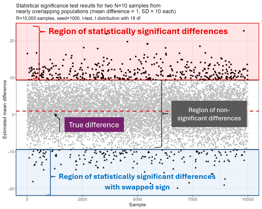
Statistical significance test results for two N=10 samples from nearly overlapping populations (mean difference Δ=1, SD=10 each sample)
But why did this happen?
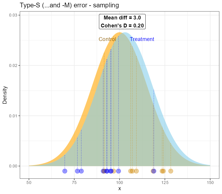
Imagine two Gaussian curves (representing population measurements of some clinical parameter) in two groups: one treated with the new therapy and a comparison group. For simplicity, let’s assume that both have the same dispersion, so they can only differ in mean. Imagine also that these distributions overlap to a large extent, almost completely. Their respective means will be very close to each other, and let’s assume that they are small enough to lead to a statistically detectable and clinically important difference (at the assumed significance level).
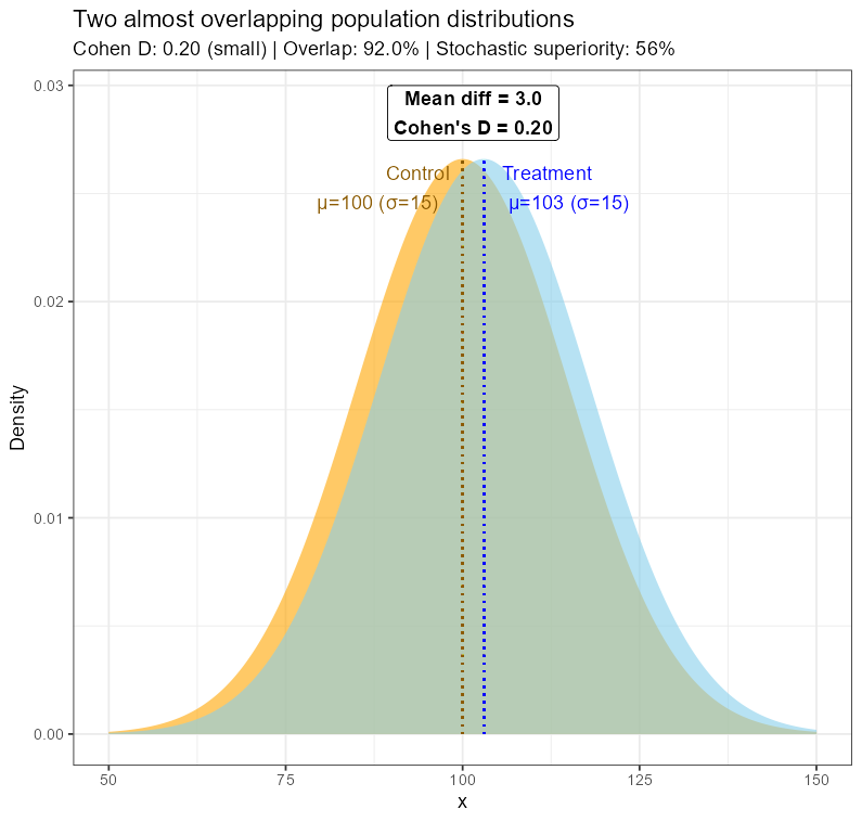
Two almost overlapping Gaussian distributions
Since we cannot see the populations, we sample from them. Now imagine that we got a statistically significant (p<0.001) and even clinically significant (>20) difference with just a few observations (say, N=10 per group).
What would have to happen to get that result? Well, if we were unlucky (I just asked R to find such a case for me 😊), we could sample our observations from areas that are close to the tails of those distributions. Of course, that can happen, since any sampling is equally possible, unless we modify the procedure in some way.
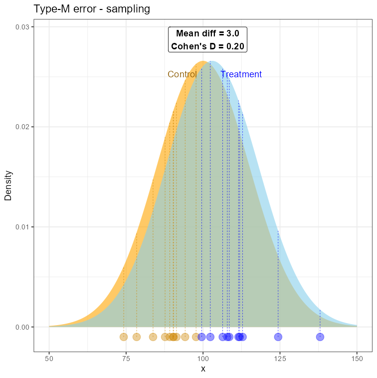
Sampling from the two nearly-overlapping distributions to demonstrate the type-M error
For small sample every observation has a greater contribution to the arithmetic mean, “pulling it” towards the extreme values. So, just by a few observations from the opposite tails, we may obtain means quite distanced from each other! This will be nothing but an artifact, not well representing the real population reality, but absolutely possible. We just experienced the type-M error. An artifact, that doesn’t speak well for the population, but the small-sample conditions made it looking real.
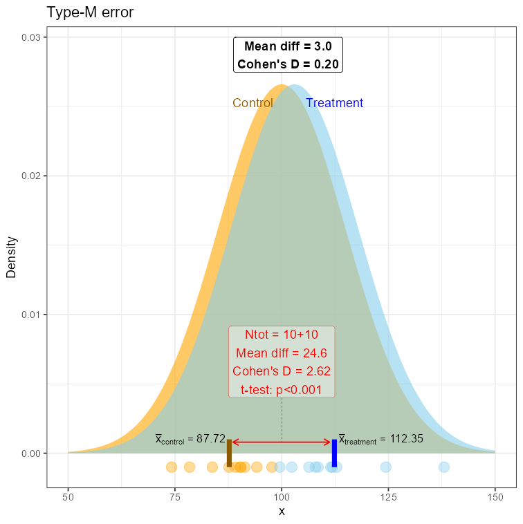
Demonstration of the Type-M error
Or even worse! The sampled data may come from opposite tails!
Sampling from the two nearly-overlapping distributions to demonstrate the type-S/M error
And this may potentially lead both to type-M and type-S errors, so not only is the effect size inflated but also the sign of the difference is now opposite (Δ=-18.5)!

Demonstration of the Type-S/M error
Well, for two reasons:
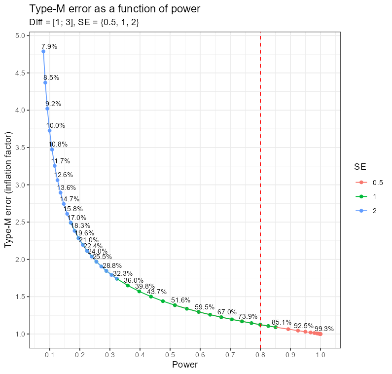
A relationship between power and the Type-M error level
A few side notes:
“With the Bayesian approach we can certainly do better. Just use a certain prior distribution to fix these problems.”
Well, yes, provided that you have the necessary knowledge. The missing information cannot be obtained out of nowhere. Both frequentist and Bayesian methods will see exactly the same data, so if the information cannot be obtained from the data or from the reliable sources (but then this problem would not even occur!), it must come from the assumptions - you will have to define somehow your prior distribution parameters, won’t you? If this knowledge is available, both Bayesians and frequentists have their tools and can address this problem appropriately. And if this knowledge is unavailable, then priors are nothing but guessing. No regularising priors, shrinkage estimators, etc will help there. In other words, no statistical “hocus-pocus” will work if you lack the domain knowledge.“Don’t use p-values, use confidence intervals!”
Well, not so easy! Confidence intervals may do no better in this case: you will still obtain the wrong magnitude of the point estimate and maybe also the sign, and the CI may lay far from 0 (p<0.0…01). The only thing that is worrying here is its length, a potential indicator of an underpowered study - but that’s all… Let’s use the data from the above examples:> t.test(control_points, treatment_points) Welch Two Sample t-test data: control_points and treatment_points t = 3.0334, df = 17.999, p-value = 0.007147 alternative hypothesis: true difference in means is not equal to 0 95 percent confidence interval: 5.701113 31.392050 sample estimates: mean of x mean of y 109.65957 91.11299The 95% CI = [5.7 ; 31.3] - and is"oddly" long (we know why!) but, at the same time, is quite far from the null value (zero). So it should immediately trigger suspicion, but one could easily claim that the effect is “discernible from zero enough", especially at so low data size…
As this topic is truly important, I recommend further reading of these articles and blog posts:
Now that we have learned about the importance of statistical power, let’s discuss some factors that, if neglected, can reduce it and compromise the entire study.
Even in short studies the number of participants at each follow-up visit may be reduced due to a variety of reasons:
The longer the study, the more likely it is that attrition will occur, both intermittent (temporary gaps in scheduled study visits) and permanent (inability to continue). Several scenarios must be carefully analysed in advance to propose effective remedies.
This naturally leads to an analysis that I call “determining the safety window” for power and sample size through simulations for alternative scenarios. One determines the minimum sample size necessary to achieve the desired power and then explores how increasing the fraction of missing observations will affect the power until it falls unacceptably low (depending on case): < 95%, 90%, 85%, and finally 80%. An example of such analysis can be found in the figure below.

This is often a truly eye-opening analysis that allows for the preparation of “emergency measures” before it is too late. In other words, it shows “how bad it can go before it IS too bad”. The more dropout scenarios we consider in our “what-if” analyses, the more the study will be “protected” against significant loss of power.
Such analyses are often skipped for several reasons, including a lack of imagination about what can go wrong, a lack of knowledge on how to conduct such simulations, or even… fear of the results of such an analysis itself plus the reactions of the decision-makers when they finally learn that additional (considerable) costs are necessary to keep the study effective.
In the example shown, the planned sample size was N=51 patients per study arm. To maintain power at above 80%, no more than 25.5% of attrition is acceptable, resulting in N=37 patients per arm.
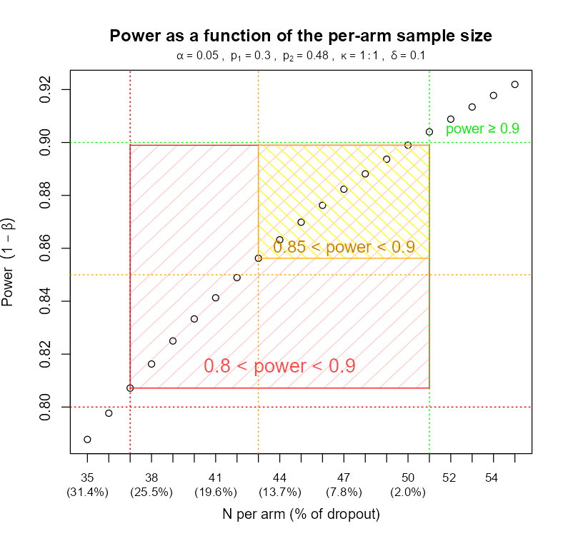
Example of a what-if power analysis (power window): a relationship between power and the fraction of dropout
Writing statistical analysis plan (SAP) is not a trivial topic. So many issues need to be anticipated, s many factor controlled and so many details – decided.
But even if the SAP is mature and specifies numerous alternatives ways of doing the analysis in presence of serious challenges, still some thigs can go wrong.
Assumptions may be disregarded or inappropriately handled.
For example, non-proportional hazards in survival analysis reduce the power of the log-rank test, which relies on the proportional hazards assumption. Similarly non-proportional odds when applying the Mann-Whitney (-Wilcoxon) or Kruskal-Wallis tests (both can be shown to be a special case of the proportional-odds model, aka ordinal logistic regression).
Another common mistake occurs when researchers apply rank-based methods (e.g., Mann-Whitney (Wilcoxon), Kruskal-Wallis) based on non-normality flagged by statistical tests such as Shapiro-Wilk, despite the data visually closely (or even indistinguishably) resembling the Gaussian distribution. In larger samples, non-normality tests quickly gain power, becominng “over-sensitive” and detecting just trivial deviations from the theoretical (non-achievable by real data!) normality that have no practical impact and are visually barely observable. If a parametric test would have been appropriate under the Central Limit Theorem, then opting for a rank-based method unnecesarily lowers statistical power. And yet we have the permutation verison of both Welch-t test and ANOVA, which not only preserve the null hypothesis (unlike rank-based methods), but also retains the power.
Oh, and by the way of mentioning the null hypothesis – rank-based methods assess a hypothesis called stochastic equivalence vs. stochastic superiority. Under non-symmetric distributions this may have nothing in common with comparing means or medians. It’s easy to find a case where Mann-Whitney would reject H0 under same means or medians and fail to reject H0 under different means or medians. And will not be a type-1 or type-2 error, this is precisely what stochastic superiority is and the test will behave exactly the way it is supposed to behave.
But! if your original objective was to test means or medians, switching to a rank-based method may affect the power of a comparison of this very kind.
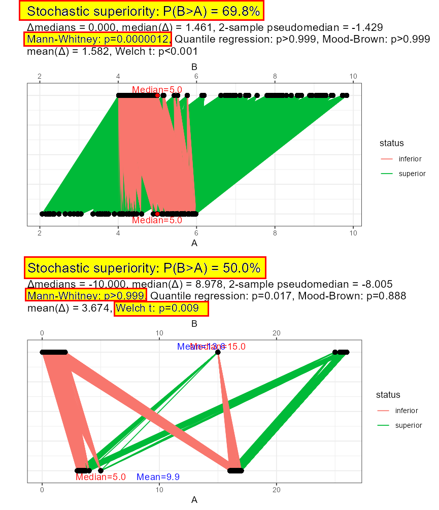
Stochastic superiority is neither about means nor medians in general
Ignored or incorrect covariate adjustments
Ignored adjustment can leave substantial residual variance unaccounted for, reducing the signal-to-noise ratio, thus lowering statistical power.
This is closely related to omitted-variable bias: if a relevant (categorical) factor that differentiates subgroups is left out, opposing effects across those subgroups may cancel each other out when averaged, producing a misleading null result. This phenomenon is conceptually similar to testing a main effect in the presence of a disordinal interaction, where simple effects have opposite signs - so when averaged, the overall effect appears negligible or absent.
Another challenge is introducing too many categorical covariates (factors) with many levels compared to the available sample size. Each level of a categorical variable “eats up” a degree of freedom, so if a covariate has many levels (say, 10) then for N=100 observations that’s 10% “spent” just on controlling for that one variable. This may, effectively, lead to unstable estimates, inflated standard errors and numerical convergence issues. By the way, this can be even more problematic if the levels are unevenly populated, i.e. some levels have very few observations. In the logistic (or multinomial and ordinal) regression this may cause the partial or complete “separation” issue.
Dichotomizing continuous variables
Turning numerical variables into categorical (e.g., splitting age into “young” vs. “old”) discards information and this may drastically reduce power. Not to mention, that the results of both descriptive and inferential analyses now depend also on the system of categorisation, e.g. the cut-off thresholds. Professor Harrell calls this “murdering data” and often this is an adequate description of this (mal)practice.
Using estimation or hypothesis testing that ignores data dependency
Doing it in studies involving repeated measurements or hierarchical (clustered) structure of observations is a serious problem. It may lead to incorrect estimation of standard errors, leading to inflated Type-1 error in some cases, and deflated power (1 minus type-2 error probability) in others if the intraclass correlation is non-negligible.

Researchers often aim to answer multiple questions in a single study, which is scientifically appealing but risky.
Not only evaluating overloading a trial with too many objectives can blur its primary focus, create internal inconsistencies, but it also complicates statistical significance control, which itself lowers the power.
This makes power analysis much more complicated, especially if the estimates are of different types (numeric, binary, ordinal, survival, etc.), require different power formulas, and the risk of missing observations is greater for some than for others, requiring additional measures to minimize their impact.
To avoid this difficulty, sponsors often choose to combine multiple goals into composite goals, the components of which are separately evaluated in binary decisions (“SUCCESS / FAILURE”) and combined using the logical conjunction operator (“AND”). However, this leads to another serious pitfall: just a single failure in the chain of the components will result in the entire goal being evaluated as a failure. Such individual failure may be a result of both true lack of effect and computational issues (such as numerical convergence error).
There are many* approaches to multiple comparisons and controlling for family-wise type 1 error probability (FWER). Unfortunately, in 2025, there still seems to be a rule ingrained in the minds of many researchers: when you ask someone to “correct for multiple comparisons,” the answer is likely to be “Bonferroni.” This is both the simplest and most conservative correction of all, penalizing a significance level higher than needed to control FWER at the desired level. Well, the simplicity of this method can be tempting and beneficial, especially at the design stage, but its conservativeness has serious negative consequences.
By “numerous” I really mean “numerous”! Let’s mention:
protected LSD (Least Significant Difference), Bonferroni, Holm(-Bonferroni), Simes, Hochberg, Šidák, Šidák-Holm, Šidák-Dunn), Hommel, Benjamini-Hochberg, Benjamini-Yekutieli, Dunn, Nemenyi, Conover, van der Waerden, Dunnett, Dunnett C, Dunnett T3, Dunnett Stepwise, Tukey + Tukey-Kramer, Tukey B, Gabriel, Games-Howel, Tamhane T2, Tamhane-Dunnett, Hochberg’s GT2, Williams, Shirley-Williams, Umbrella-protected Williams, Dermott, Marcus, Marcuss-Umbrella protected, GrandMean, Ryan-Einot-Gabriel-Welsch F and Q, Student-Newman-Keuls (SNK), Duncan Multiple Range Test (MRT), Waller-Duncan, Scheffe, Ury-Wiggins-Hochberg, Dwass-Steel-Critchlow-Fligner, Cuzick, Johnson-Mehrotra, Skillings-Mack, Waller-Duncan, Siegel, Miller, Conover, Conover-Inman, Demsar, Fixed sequence procedure, Fallback procedure, Gatekeeping (serial, parallel), Sequential online: [LOND, LORD (++, 3, D), SAFFRON, Alpha-investing, ADDIS + A.-spending], Online FDR, adaptive methods (O’Brien-Fleming, Pocock, Haybittle-Peto, DeMets) and this doesn’t end here!
To explain the problem, let’s first recall the simplified formula explaining the power of the simplest 1-sided z-test below. The level of significance (α) is “plugged in” into the critical value of the test statistic, which determines the power. As we lower α (which is exactly what the multiplicity adjustments do!), the critical value moves further into the right tail of H₀. Both H₀ and H₁ are still overlapping in their opposite tails, but now less of H1 mass lies beyond the new critical value. That means less power.
Think of it this way – if you wanted to account for testing multiple hypotheses when designing your study, the significance level would be lower (e.g., α divided by the number of comparisons). To hold β (type 2 error probability), effect size, and variance constant, the minimum number of patients to recruit would increase. Or you could keep the sample size the same, but then something else would have to change… either you need a larger effect, smaller variance, or… allow for less power! See? No free lunch!

Power as a function of statistical significance in the context of multiplicity adjustments
So, although Bonferroni is simple, we may need something more sophisticated to minimize its impact on power. Ideally, we would like to test multiple hypotheses with minimal penalty on significance level (α) - or even better - unchanged (yes, this IS possible).
And indeed, improvements are possible. Holm adjustment makes no assumptions about the hypotheses (just like Bonferroni) and is uniformly more powerful than Bonferroni! Hommel and Hochberg offer further improvement but also make some non-trivial assumption - namely they are valid when the hypothesis tests are independent or when they are non-negatively associated.
For model-based hypothesis testing and interval estimation, there is also a parametric step-up correction based on the multivariate t-distribution (hence the name: MVT), using both the estimated model coefficients and the covariance matrix estimator. It is implemented in the R statistical software in the multcomp and emmeans packages.
Now, if you can prioritize the hypotheses and organize them into a hierarchy, then you can use more modern sequential methods such as fallback or fixed-sequence, and the “penalty” can be much smaller than with the Bonferroni method, or even not necessary at all, as long as all hypotheses in the chain are rejected. Thus, power is largely preserved or fully regained.
The theory of multiple comparison procedures (MCP) and closed testing procedures (CTP) has evolved significantly since their initial development, with major contributions by researchers such as Bretz, Tamhane, Dmitrienko, and Wiens. Their work provides a solid methodological framework by formalizing principles for distributing and controlling the significance level across multiple hypotheses, particularly in complex testing scenarios like gatekeeping and adaptive designs. It resulted in a set of flexible adjustment methods:
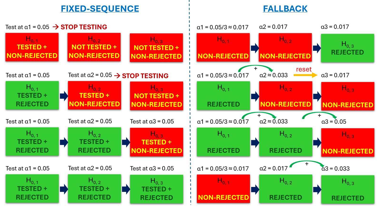
An idea of the two common sequential multiplicity adjustments: fixed-sequence and fallback
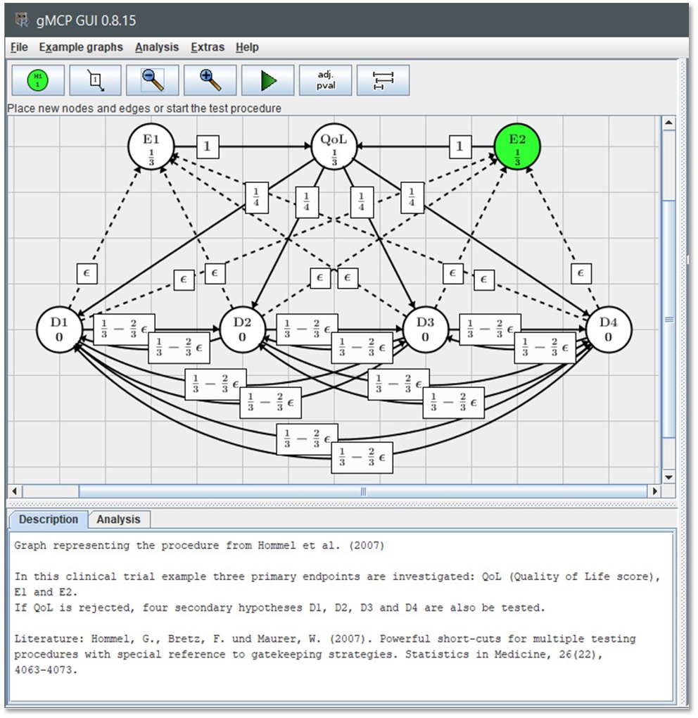
The graphical method enables a new level of flexibility in controlling the FWER
Curious readers may find more information in the following books:
By the way, R has numerous packages offering these methods: multcomp, emmeans, gMCP ( check this PDF too ), Mediana, multxpert, to name a few.
Embedding practical importance into the tested hypothesis, e.g. in clinical superiority studies, using a 1-sided, directional hypothesis about some Minimal Clinically Important Difference (MCID) requires accounting for this quantity during the power analysis.
Statistical significance only tells us whether the observed data are incompatible with a null hypothesis (e.g., a difference of 0 or a ratio of 1). When we reject the null, the confidence interval (CI) around the effect estimate excludes that null value - but it might still include values that are statistically different from zero but clinically trivial. This is shown in the left panel of the figure showed below: although the CI excludes 0 (so the result is statistically significant), it still includes small values close to zero, indicating a possible effect that may be too small to matter clinically.
In contrast, a clinically meaningful result is shown in the right panel, where the entire confidence interval lies beyond the MCID threshold. This suggests that not only is the effect statistically significant, but it also exceeds the minimum level of importance for clinical decision-making.
To properly design such (e.g. superiority) study focusing on detecting a clinically relevant effect, one must incorporate the MCID into the effect size used for sample size calculation. This usually requires a larger sample size than what would be needed to merely detect any non-zero difference.
If the MCID is ignored in the design phase, the study may end up being statistically powered to detect negligible differences, but underpowered to detect differences that actually matter to patients or clinicians.
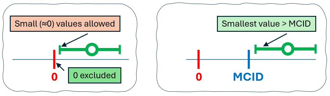
The difference between result statistically significant and statistically-practically significant
Well, this chapter will be just a one-liner: using small pilot studies to inform power calculations is risky, because underpowered studies may yield inflated or even directionally wrong effect estimates (remember the Type-M and Type-S errors?), which can mislead and compound design flaws in subsequent trials. So the issues will “propagate” further and further.
Even if a clinically important effect size can be somehow agreed between the domain specialists, trial design still requires a (realistic!) estimate of variability. So even if clinicians can define the minimal difference that would be important in practice, they may have little or no intuition about the underlying population variance. This is crucial because the signal-to-noise ratio determines how easily such an effect can be detected and how many subjects are necessary for that. Unfortunately, estimates of variability from small pilot studies can be “unstable,” i.e., standard deviations can vary greatly across small samples, leading potentially to underestimated number of patients required. It would be best to combine estimates from previous studies, if only available, with existing knowledge about the domain. The “what-if" analyses can also shed some light on it. But if the study is pioneering, such data may simply not yet be available, and then all that is left is guesswork (whether in a frequentist or Bayesian framework).
For decades, we have been told how important it is to ensure that the study has adequate statistical power to detect a given effect. In our article, we have shown that the lack of statistical power can have far greater consequences than is typically discussed, resulting in fake exaggerated effects (even with the wrong sign!) that easily reach statistical and even clinical significance. We have also described a few factors that can negatively affect the level of statistical power, showing how complex this issue is and how easy it is to fail a study due to ignorance or carelessness in treating these topics.
Dare to risk it?
To be continued…


If you’re thinking of your study design audit or rescue action contact us at or discover our other CRO services .
🔥HOT NEWS!!!🔥 We’ve just released our brand new eCRF platform GoResearch™.live , available also in SaaS model. Check it out on its web page or news section.
2KMM Sp. z o.o.
ul. Strzelców Bytomskich 3
40-310 Katowice
Polska / Poland


